AeVP: Peeling Back the Layers of Autoencoders

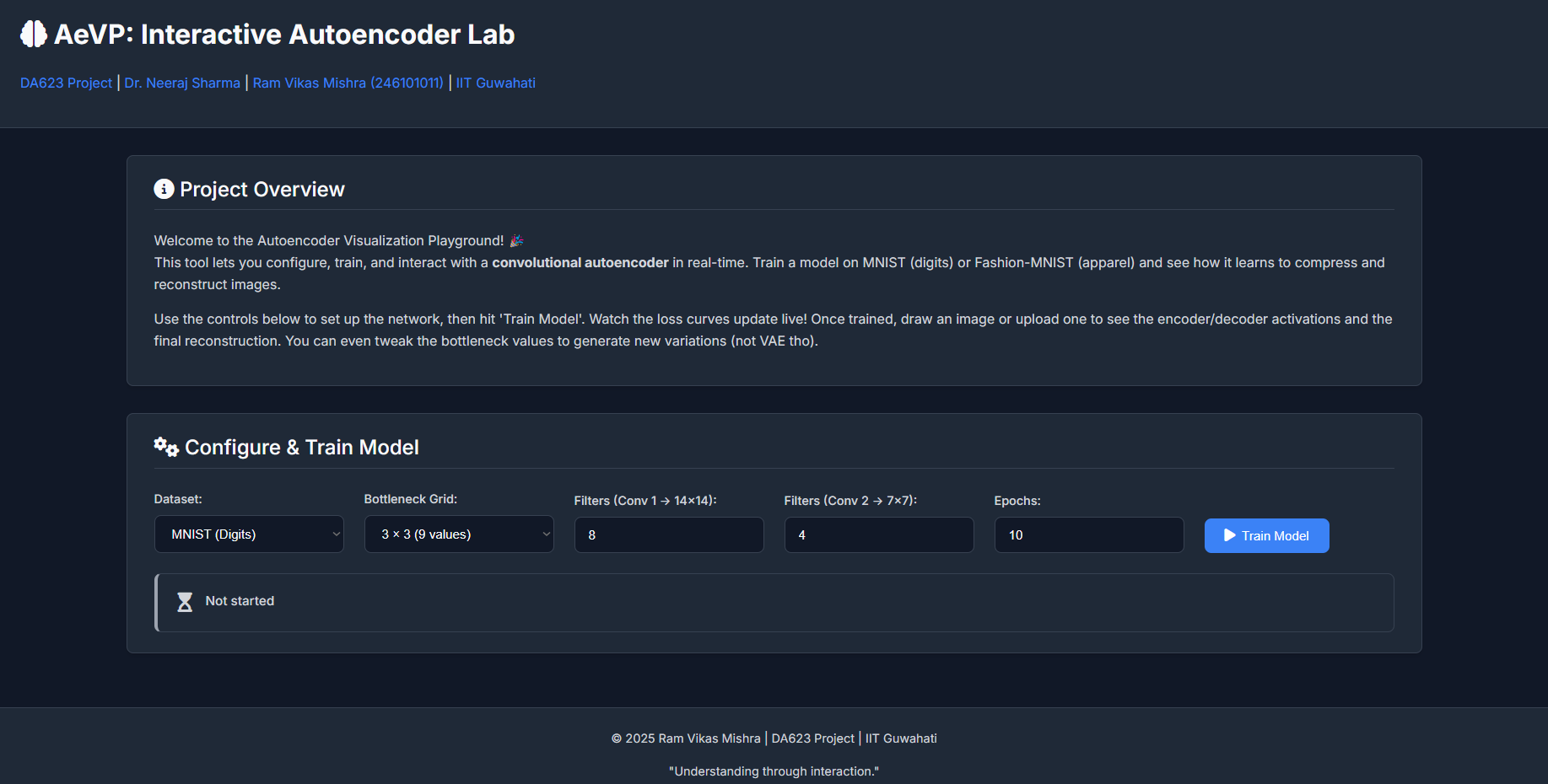
Neural networks, particularly deep learning models, often feel like intricate "black boxes." We feed them data, they produce outputs, but what happens in between? This project, the AutoEncoder Visualization Project (AeVP), developed for the DA623: Computing with Signal course, aims to demystify one such fascinating architecture: the Convolutional Autoencoder.

Motivation – Why Autoencoders?

My fascination with autoencoders stems from their elegant simplicity and profound capabilities. The core idea of compressing data into a lower-dimensional "latent space" and then reconstructing it back isn't just a clever trick; it's fundamental to unsupervised learning, dimensionality reduction, feature extraction, and even generative modeling. For a course titled "Computing with Signal," understanding how signals (in this case, images) can be efficiently represented and transformed felt like a perfect fit.

Dr. Neeraj Sharma, our instructor, is known for his engaging teaching style that emphasizes building strong intuition. This project was conceived in that spirit: not just to implement an autoencoder, but to create an interactive tool where one can *see* it learn, *play* with its internal representations, and thereby gain a deeper, more intuitive understanding of its mechanics.

Connection with Multimodal Learning

While AeVP focuses on unimodal data (images from MNIST or Fashion-MNIST), the principles of autoencoders are foundational to many advanced multimodal learning systems. Multimodal learning deals with integrating and processing information from different types of data sources (e.g., text, images, audio). Here's a brief perspective:

• Shared Latent Spaces (Early to Mid-2010s): Early multimodal work often involved training separate autoencoders for each modality and then trying to align their latent spaces. The goal was to find a common, compact representation where, for instance, the image of a "cat" and the word "cat" would map to nearby points. Models like DeepCCA or bimodal autoencoders explored this.
• Cross-Modal Generation & Translation (Mid-2010s to Present): Autoencoders, particularly Variational Autoencoders (VAEs) and Generative Adversarial Networks (GANs) (which share conceptual similarities in learning data distributions), became crucial for tasks like generating images from text descriptions or vice-versa. The encoder learns to capture the essence of one modality, and the decoder (sometimes conditioned on another modality) learns to reconstruct or translate.
• Transformers & Self-Supervision (Late 2010s to Present): The rise of Transformer architectures (like BERT, GPT, ViT) revolutionized the field. While not always "autoencoders" in the classic sense, their pre-training objectives often involve self-supervised tasks akin to masked autoencoding (e.g., predicting masked words in text or masked patches in images). This allows models to learn rich representations from vast amounts of unlabeled multimodal data. Recent models like CLIP (OpenAI) learn joint image-text embeddings by contrasting positive and negative pairs, effectively finding a powerful shared latent space. DALL-E and Stable Diffusion use encoder-decoder like structures within complex diffusion models to generate high-fidelity images from text.

AeVP, by providing intuition on how an encoder compresses information into a latent space and how a decoder reconstructs from it, offers a stepping stone to understanding these more complex multimodal systems. The core idea of a "bottleneck" representation is a common thread.

My Learning Journey with AeVP

Building AeVP was an incredibly enriching experience, far beyond just coding a neural network. Here are some key takeaways:

1. The Power of Interactive Visualization: Simply looking at loss curves is one thing; seeing activation maps change as you draw a digit, or tweaking bottleneck sliders and observing the reconstructed image morph in real-time, provides a visceral understanding of what the network is "seeing" and "thinking."
2. Hyperparameter Sensitivity: The interactive configuration panel immediately highlighted how sensitive autoencoders are to choices like the number of filters and the latent dimension size. Too small a bottleneck, and the reconstruction quality suffers; too many filters in early layers without a correspondingly complex task might not always improve things significantly and increases training time.
3. Feature Hierarchy: Observing the activation maps from the first convolutional layer versus the second showed a clear progression. Early layers often learn simple edge detectors or basic texture patterns. Deeper layers (before the bottleneck) combine these to form more complex, abstract features representative of parts of digits or apparel items.
   
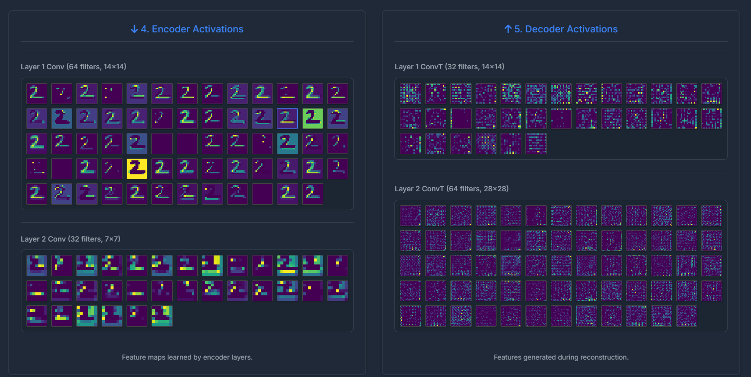
4. The "Meaning" of Latent Space: While individual neurons in the bottleneck might not always correspond to easily interpretable semantic features (e.g., "top loop of a 5" or "sleeve of a shirt"), the *collective* activation pattern in the latent space clearly encodes the "essence" of the input. Manipulating these values often leads to plausible (though sometimes novel) variations of the input class. This hints at the generative capabilities of autoencoder-like structures.
   
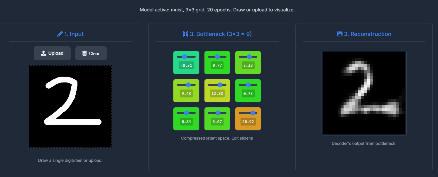
5. Backend-Frontend Integration Challenges: Managing asynchronous training in a background thread while providing real-time status updates to a Flask-served frontend, all within a Colab environment, was a good lesson in practical MLOps. Handling state (like the currently active model configuration) consistently between the backend and frontend required careful design.
6. UI/UX for Explainability: Designing the UI wasn't just about aesthetics; it was about making the complex process understandable. The flow from configuration to training status, then to the input-encoder-bottleneck-decoder-output pipeline, was intentional to guide the user through the autoencoder's operation. The new UI aims for clarity and a modern feel.

Code / Notebook – AeVP in Action

The entire project is implemented as a single Google Colab Notebook. This allows for easy setup and execution, as all dependencies are installed and the Flask web server is run within the Colab environment.

Launch AeVP in Google Colab

Key Code Snippets & Experiments:

While the full code is in the notebook, here are a few illustrative Python snippets:

1. Dynamic Model Building:

The core autoencoder architecture is built dynamically based on user configuration passed from the frontend.

# (Simplified from the notebook)
def build_autoencoder(config):
    latent_grid = config['latent_grid']
    latent_dim = latent_grid * latent_grid
    filters_stage1 = config['filters_stage1']
    filters_stage2 = config['filters_stage2']
    input_shape = (28, 28, 1)

    # Encoder
    encoder_inputs = Input(shape=input_shape, name='encoder_input')
    x = layers.Conv2D(filters_stage1, (3,3), activation='relu', padding='same', strides=2, name='encoder_conv1')(encoder_inputs)
    x = layers.Conv2D(filters_stage2, (3,3), activation='relu', padding='same', strides=2, name='encoder_conv2')(x)
    # ... flatten and dense to bottleneck ...
    encoder_outputs = layers.Dense(latent_dim, name='bottleneck')(x)
    encoder = models.Model(encoder_inputs, encoder_outputs, name='encoder')

    # Decoder
    decoder_inputs = Input(shape=(latent_dim,), name='decoder_input')
    # ... dense, reshape, Conv2DTranspose layers ...
    x = layers.Conv2DTranspose(filters_stage1, (3,3), activation='relu', padding='same', strides=2, name='decoder_convT2')(x)
    decoder_outputs = layers.Conv2D(1, (3,3), activation='sigmoid', padding='same', name='decoder_output_conv')(x)
    decoder = models.Model(decoder_inputs, decoder_outputs, name='decoder')

    autoencoder = models.Model(encoder_inputs, decoder(encoder_outputs)) # For training
    return encoder, decoder, autoencoder
            

This flexibility allows for quick experimentation with different architectural choices without rewriting code.

2. On-Demand Training and Status Updates:

Training is triggered via a Flask endpoint and runs in a background thread. A Keras callback updates a global status dictionary, which the frontend polls.

# (Simplified training thread logic)
class TrainingStatusCallback(callbacks.Callback):
    def on_epoch_end(self, epoch, logs=None):
        with status_lock:
            training_status["current_epoch"] = epoch + 1
            training_status["loss"] = logs.get('loss')
            training_status["val_loss"] = logs.get('val_loss')
            # ... (update message)

# In Flask route /train:
# training_thread = threading.Thread(target=train_model_thread, args=(config,))
# training_thread.start()

# In Flask route /train_status:
# return jsonify(training_status)
            

3. Visualizing the Training Curve:

After training, the loss and validation loss history are sent to the frontend and plotted using Chart.js. This gives immediate feedback on model convergence and potential overfitting.

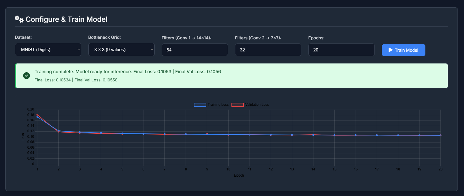
Experimenting with different learning rates (though not configurable in this UI version), filter sizes, and bottleneck dimensions directly impacts this curve. A smaller bottleneck, for instance, might lead to higher reconstruction loss as the model struggles to compress information adequately.

4. Bottleneck Manipulation:

The most "fun" part is editing the bottleneck values. When a user draws a '7', the encoder produces, say, 9 values for a 3x3 bottleneck. The UI displays these as sliders. Changing one of these slider values and seeing the reconstructed image morph into something that might be "7-like" but slightly different, or even transition towards another digit if a value is changed drastically, is highly instructive. It demonstrates that the latent space has learned some continuous representation of digit features.

Reflections

(a) What surprised you?

• Robustness of Learned Features: Even with relatively few filters (e.g., 8 in the first conv layer, 4 in the second) and a small number of epochs (10-15), the autoencoder could learn meaningful features and produce recognizable reconstructions. This highlights the efficiency of convolutional layers for image data.
• Interpretability of Some Activation Maps: While not all filter activations are humanly interpretable, some clearly corresponded to specific strokes, curves, or corners, especially in the earlier layers. This was more apparent with MNIST than Fashion-MNIST, which has more complex textures.
• The "Smoothness" of the Latent Space: Small changes in the bottleneck sliders generally led to smooth, continuous changes in the output image, suggesting the model learned a somewhat well-behaved manifold for the data.
• Colab & Flask Nuances: Running a multi-threaded Flask application within Colab, especially one that modifies global state (the active models), required careful handling of threads and ensuring `use_reloader=False` for stability.

(b) What can be the scope for improvement?

• More Advanced Architectures: Incorporate options for ResNet blocks, attention mechanisms, or even a Variational Autoencoder (VAE) to explore generative capabilities and probabilistic latent spaces.
• Quantitative Evaluation: Display quantitative metrics like PSNR, SSIM, or Mean Squared Error for the reconstructions alongside the visual output.
• Latent Space Visualization (t-SNE/UMAP): Add a 2D scatter plot of the bottleneck representations of a batch of test images, colored by their true labels. This would visually demonstrate how well the encoder clusters similar classes in the latent space.
• Conditional Generation: For a VAE, allow users to sample from the latent space (perhaps by clicking on the t-SNE plot) to generate new images.
• More Datasets: Extend to slightly more complex datasets like CIFAR-10 (though color would add complexity).
• Hyperparameter Tuning UI: Allow configuration of learning rate, optimizer, and activation functions.
• Pre-trained Models: Offer a selection of pre-trained models for different configurations so users can immediately start visualizing without waiting for training every time.
• Deployment Beyond Colab: Package the application for easier standalone deployment (e.g., using Docker).

References

This project drew inspiration and technical knowledge from various sources:

• Core Concepts:
  • Goodfellow, I., Bengio, Y., & Courville, A. (2016). Deep Learning. MIT Press. (Specifically chapters on Autoencoders and Representation Learning).
  • Chollet, F. (2017). Deep Learning with Python. Manning Publications. (Keras examples and explanations).
• Autoencoder & Visualization Tutorials:
  • TensorFlow/Keras Official Tutorials on Autoencoders: (tensorflow.org)
  • Various blog posts and articles on building autoencoders and visualizing activations (e.g., on Medium, Towards Data Science).
• Dataset Sources:
  • MNIST: Yann LeCun's MNIST Database
  • Fashion-MNIST: Zalando Research's Fashion-MNIST GitHub
• Web Technologies & Tools:
  • Flask Documentation: flask.palletsprojects.com
  • Chart.js Documentation: chartjs.org
  • MDN Web Docs (HTML, CSS, JavaScript): developer.mozilla.org
  • Google Colaboratory: For the interactive development environment.
• LLM Assistance:
  • Google's Gemini: Used for brainstorming UI/UX ideas, generating boilerplate HTML/CSS/JS for the modern UI, refining explanations, and assisting with debugging Python and JavaScript code, especially for the Flask/threading integration within Colab and the Chart.js implementation. It was particularly helpful in quickly scaffolding the new UI structure based on descriptive prompts.

"The best way to understand autoencoders is to build one yourself and see it in action!"